RECOMMENDER SYSTEMS
TYPE SYSTEMS
Rust
BANDITS
Game Theory
DEEP LEARNING
PROGRAMMING LANGUAGE THEORY
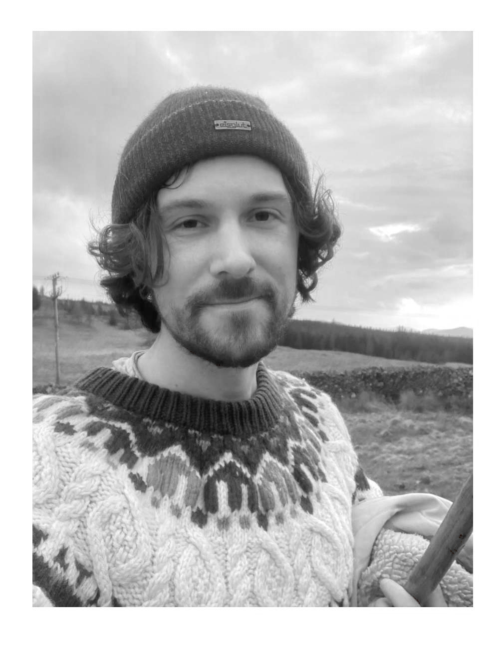
Hi! I'm Leon Luithlen, the person this page is about.
You can get a sense of my interests from the little topic introductions above. I am currently working on Sistema Labs to bring transformer models to fields other than nlp at scale. This is also where you will find my recent open source work, while the blog posts below summarize a research project I developed in 2020-2021.
If you are interested in my professional profile, you can have a look at my linkedin.
If you feel like I could be of help, or you want to discuss anything in particular, you can go through linkedin or write to (all lowercase):
[first name][middle name][last name] @ [google email service] .com
My middle name is Timna. Please reach out!
The adaptive ensemble (implemented in the library “AdaEnsemble”) consist in a multi armed bandit algorithm that chooses between different machine learning models, and passes the data passed to the ensemble down to the selected machine learning model. The output of the selected model, given the data, is the output of the ensemble. Here are three patterns by which adaptive ensembles might be applied. Importantly, the member models of each ensemble can be from any family of machine learning models, if they produce an output that can be used to calculate a reward. This straightforwardly includes all supervised learning algorithms and reinforcement learning.
The chart bellow illustrates the composition of an adaptive ensemble.
Three patterns of how the adaptive ensemble might be used can be found here.
A technical introduction to the AdaEnsemble library that implements the adaptive ensemble can be found here.
An empirical demonstration of the application of an adaptive ensemble, to address machine learning pipeline underspecification, can be found here.
Yes, you can! It can be found here.
AdaEnsemble is a library for building adaptive ensembles, which consist in a multi armed bandit algorithm choosing among machine learning models and gradually learning which ML model is best, or best given a particular context. These ensembles consist of an Ensemble object which “contains” two or more Model objects and an equal number of Distribution objects that contain the representation of the reward associated with each model. This document will outline the specifics of different types of ensembles, models and rewards, and updated as the library expands.
The library “AdaEnsemble” contains three broad types of ensembles: “stackable” ensembles of types 1 and 2, and contextual ensembles.
All three types of ensembles are stackable: they can contain other ensembles as models. This results in a hierarchy of ensembles, each choosing (on selection by the layer above) a member model, which can be an ensemble in its own right or another kind of model. The only limitation is that “stackable” ensembles of types 1 and 2 cannot be mixed with contextual ensembles.
Ensemble type | Description |
---|---|
Stackable ensemble of type 1 | Model selection does not depend on data |
Stackable ensemble of type 2 | Model selection depends on data |
Contextual ensemble | Model selection depends on a context different from the data passed to the selected Model object |
The different elements of an adaptive ensemble (Ensemble object, Models and Distributions that represent rewards) are tied together by type parameters. The five type parameters, of which not all apply to every object are ModelID, Context, ModelData, ModelAction and AggregateReward.
These type parameters structure the library as a whole, and putting together an adaptive ensemble usually requires that they match for the different components.
Constraints on type parameters
Ensembles that use unconditional Thompson Sampling are constrained to employ an AggregateReward that is a BetaDistribution, and Ensembles that use conditional Thompson Sampling are constrained to use BayesianSampleRegressionDistribution.
So far, three kinds of models are available:
The most versatile of these are the onnx models, as they enable the incorporation of all or almost all machine learning models developed and trained in scikit-learn, TensorFlow, PyTorch, and many other machine learning frameworks. The only downside is that onnx does not allow continued training of the models – onnx models are static.
Constraints on type parameters
Models impose constraints on the type parameter values that are available to an ensemble. They are summarised in the following table.
Static models | No constraints |
---|---|
Onnx models | In OnnxTensor.createTensor(env, data), data is of type ModelData and must be compatible with the createTensor function |
Bayesian regression models | ModelData must be of type Array[Double] and ModelAction of type Double |
Distribution is the type any representation of the reward associated with a model must take. Such a representation can either be a SimpleDistribution in case the reward does not depend on any data, or a ConditionalDistribution[A] in case it does.
The available implementations of SimpleDistribution are the following:
The available implementations of ConditionalDistribution are the following:
Constraints on type parameters
ConditionalDistribution impose the constraint that the type parameter Context it takes is a subtype of Array[Double]. For a contextual distribution, the ensemble type parameter Context must thus be a subtype of Array[Double], while for a stackable ensemble of type 2, ModelData must be a subtype of Array[Double].
Here, for example, is the way to create an epsilon-greedy ensemble, which picks the model with the highest reward with probability (1 – epsilon) and randomly one of the others with probability epsilon. The ModelID type is Int, the ModelData type is Array[Double], the ModelAction type is Double and the reward distributions is MeanDouble.
1. Create a static model, which always returns the same value:
new StaticModel[Int, Array[Double], MeanDouble](0.0)
2. Create a bayesian regression model:
new BayesianMeanRegressionModel[Int, MeanDouble](5, alpha=0.3, beta=5.0)
3. Create the rewards:
List(new MeanDouble, new MeanDouble)
4. Create the ensemble:
new GreedyEnsemble[Int, Array[Double], Double, MeanDouble](
models=(i: Int) => modelsMap(i),
modelKeys=() => List(0, 1),
modelRewards=rewards,
epsilon= 0.3)
My hope is that the hierarchical combination of exploratory multi armed bandits with fixed or slowly evolving neural and other machine learning algorithms has many applications.
Three I have thought of:
The adaptive ensemble (implemented in the library “AdaEnsemble”) consist in a multi armed bandit algorithm that chooses between different machine learning models, and passes the data passed to the ensemble down to the selected machine learning model. The output of the selected model, given the data, is the output of the ensemble. Here are three patterns by which adaptive ensembles might be applied. Importantly, the member models of each ensemble can be from any family of machine learning models, if they produce an output that can be used to calculate a reward. This straightforwardly includes all supervised learning algorithms and reinforcement learning.
A Brief Note On Charts
In the charts that follow, each line represents a model that can be chosen by the ensemble, and the line thickness represents whether a model is more or less likely to be picked by the ensemble. They have been created purely for illustrative purposes and do not show the actual mechanics of an ensemble, which depend on many factors and make consise visualisation pretty difficult.
1. Online model selection on static models: the adaptive ensemble picks the best model of two or more machine learning models. The models do not adapt to new data, but the ensemble reacts to feedback and applies the model that is better at a given time.
In the example, the generating process consists in either returning a constant value or a sine transformation of that value, but always one or the other for prolonged stretches of time. The two lines represent two models that were trained on prior data. These models do not change with incoming data, but the adaptive ensemble learns to pick the better model given recent feedback. The likelihood of a model being picked by the ensemble is represented by the thickness of the line.
An example with convolutional image classifiers in the case of pipeline underspecification can be found in the post on mitigating pipeline underspecification.
The ensemble starts out picking the linear model, then changes to pick the sinusoidal model after the data changes so that it fits better, and then reverts to the linear model as the data changes yet again.
2. Incremental learning with insurance: the adaptive model contains one or more incremental machine learning models and one or more static models. The incremental learners can adapt to new data, but in case they diverge or perform worse than the alternative static model for another reason, the ensemble can choose to go back to the static model. In this way, incremental learning might be introduced to a use case with the knowledge that in the worst case the ensemble reverts back to the established static model.
At first, the static model conforms well to new data, and is picked most frequently by the ensemble (represented by the thicker line). Then, the data generating process changes and the incremental learning proves superiour, and thereby is selected more frequently by the ensemble. Towards the end, it changes again and the static model performs better again, and the ensemble switches back to using the static model.
The ensemble starts out relying mainly on the static model trained in advance. As the data changes, the incremental linear regression starts to fit the data better, and it is chosen more frequently by the ensemble. Then, the data reverts to its previous behaviour and the ensemble returns to the static model.
3. Online hyperparameter tuning: an incremental learning algorithm might take have multiple hyperparameters that need to be set at the outset. Algorithms with different settings can just be bundled into an adaptive ensemble, which will learn to apply the model with the best available hyperparameters. In this example, the hyperparameter is the number of previous data points that are used for regression, and the the regression based on a longer horizon proves superiour, and is selected by the ensemble.
The ensemble starts out choosing both incremental linear regression equally often, and then converges on the model with the longer training horizon, as it proves more accurate in its predictions.
A technical introduction to the AdaEnsemble library can be found here.
The recently published paper “Underspecification Presents Challenges for Credibility in Modern Machine Learning” by researchers at Google including Alexander d’Amour, Katherine Heller and Dan Moldovan brought the issue of underspecification in machine learning pipelines to the attention of the ML community. In its newly refined definition, underspecification in supervised learning consists in model architectures and training schemes that can lead to multiple models with equivalent performance on held-out data, but different performance on new data. This divergence is due to different inductive biases encoded in these models. In this post I want to propose a mitigation strategy that might be of use in some circumstances where underspecification is a problem. It consists in training multiple models with a given pipeline and choosing between them in production with a multi armed bandit (MAB) algorithm, updating the parameters of the MAB model by the loss incurred by the predictions of the model of the underlying arm. This ensemble based on a MAB model choosing between arms that are themselves machine learning models might be called “adaptive ensemble”.
A supervised learning task consist in finding a predictor f : X → Y that takes inputs x to outputs y, where x can consist of any kind of data, such as images, text, sociodemographic or behavioural data, and y is either a label or a real number. A machine learning pipeline is underspecified when the class of predictors F from X to Y contains a subclass F* with equivalent (i.e. optimal or near optimal) performance on held-out data and substantially different inductive biases, leading to different performance on new, differently distributed data (a more expansive introduction to the problem can be found in the original paper , which you should read!) . In choosing a predictor f from F*, a pipeline cannot assess the usefulness of its inductive biases on new data, and might choose a predictor that is suboptimal in that setting.
MAB algorithms are a class of algorithms that optimise the repeated choice among a given set of alternative actions under uncertainty. Given a set of real distributions B = {R1,…, RK} , with each representing the reward associated with one of K alternative actions and mean values μ1,…, ,μK , the MAB algorithm repeatedly chooses an action j in K and observes a reward value drawn from Rj. MAB algorithms aim to maximise the total reward by choosing the action associated with the highest value in μ1,…, ,μK as often as possible. The difficulty lies in not knowing in advance which action that is. The trade-off between learning with more certainty which action is best and choosing the action that seems best so far is called the explore-exploit dilemma.
MAB algorithms can be characterised by different ways of 1) representing the reward associated with each action 2) choosing the next action and 3) updating the representation of the reward associated with the chosen action given the observed reward value. For example, a simple and often effective MAB algorithm is the Epsilon-Greedy Algorithm, which represents rewards by their observed mean, chooses the action with the highest observed mean with probability (1 – ε) and one of the other actions at random with probability ε, and updates the observed mean associated with the action taken by taking the weighted average of its prior value and the observed reward value.
Maybe the obvious approach to the problem of underspecification is to select a subset of F* and try them out in the area of application to see which one performs best. Using an adaptive ensemble is a way of implementing this approach while circumventing additional demands on researcher time and attention. Instead of waiting on new data from the application domain and evaluating the alternatives on it, selecting the best one, the researcher can delegate this process to the MAB algorithm.
This approach has other benefits: MAB algorithms make optimal choices in the face of the explore-exploit dilemma, which in this instance consists in using the model that appears best so far, and trying out other models to collect information on their performance. Depending on the specific MAB algorithm, it also leaves the door open to adaptation to further data drift: at some later stage, a different model in the set of alternatives might have optimal inductive biases, and in an adaptive ensemble, that change can be detected and acted upon automatically. These things are achieved while the computational cost of inference is kept nearly constant relative to choosing a model in F* at random. However, it also has several disadvantages, the biggest of which is the necessity to calculate a reward or a correct output for predictions in production, which is necessary to train the MAB algorithm. Additionally, there is the need to define MAB hyperparameters, higher memory usage, and a higher uncertainty relative to the manual approach as to the performance achieved in the wild.
However, in cases where a reward can be readily calculated, it seems to me that it strikes a good balance between the current norm of choosing a member of F* and leaving it at that, and manual model selection on new data. It improves on the first by making convergence on the optimal member of the alternatives (a subset of F*) exceedingly likely, compared to a random and therefore likely suboptimal choice from F*, at the cost of some researcher effort and computer memory. It improves on the second by enabling ensemble definition in advance, before any new data is collected, saving researcher time, increasing resilience to future data drift and adding explore-exploit optimisation.
These characteristics make it appropriate for applications with moderate stakes, where no guarantees on performance on new data are necessary. In such applications, a set and forget deployment of an adaptive ensemble should improve on randomly selected model (in F*) at a moderate cost. It might also be preferable to manual evaluation in a high stakes setting where model deployment cannot be held off while its performance on new data is evaluated. In such a case it would need close monitoring, and lose its researcher time advantage, but might still be desirable for its explore-exploit optimisation.
In general, it is possible to set the reward function for the MAB algorithm to be identical to the one used to train the individual models. In that case, the adaptive ensemble is in some sense an extension of the original training process, minimising expected error.
However, it might also be put to more creative use. In the d’Amour et al. article, the authors note that “these solutions [to a single learning problem specification] may have very different properties along axes such as interpretability or fairness.” The reward function for the MAB algorithm is not limited to accuracy metrics. This opens up the possibility of incorporating algorithmic fairness, plausibility of feature contributions to outcomes, legal requirements on decision processes and any other criterion that might be relevant to a particular application.
The idea to use MAB algorithms for online model selection is possibly quite widely known, but there is nonetheless surprisingly little published research on this topic. A subset of the Active Learning literature seems to employ MAB algorithms as meta algorithms (eg here ), and a recent paper applies Thompson Sampling on recommender systems with promising results. However, it does not appear to be a widely established technique in applied settings.
I am currently developing the Scala library AdaEnsemble to enable the
simple creation of adaptive ensembles. It still under development but
with an API that is basically fixed, and I will briefly show how it can
be used. In the example, an adaptive ensemble is used to select the
ResNet image classification model which generalises best for the
categories “people” and “furniture” in the dataset CIFAR100.
The ResNet models are trained in PyTorch and stored in the ONNX format, and loaded into the Scala model using onnxruntime. The AdaEnsemble library can load a classification model from the path to the ONNX file like this:
new OnnxClassifier[Int, Array[Array[Float]], Int](PATH_TO_FILE, "input", i => i)
Then, an adaptive ensemble can be defined as follows. In this case a
ThompsonSampling model is used with initial alpha and beta values of 1,
and five models contained in a List:
new ThompsonSamplingEnsemble[Int, Array[Array[Array[Array[Float]]]], Int]( (0 until 5).zip(models).toMap , 1, 1)
This ensemble can then be used by taking an action (in the case of a
predictive model that means making a prediction) and updating the MAB
alrgorithm (in this case Thompson sampling), as follows:
val (action, modelIds) = ensemble.actWithID(data, List())
and
ensemble.update(modelIds, reward)
Model initialisation, ensemble initialisation, taking an action and
updating are all the operations that are necessary to employ an adaptive
ensemble.
I have trained five ResNet image classifiers initialised with different seeds on a subset of CIFAR100 images. The CIFAR100 dataset includes fine and coarse labels, consisting of 100 fine categories and 20 coarse ones. Every fine category is a strict subset of a coarse category. To emulate real world data drift I trained the image classifiers on three out of five fine categories for every coarse category with the coarse category as target, and used the trained models on the remaining two fine categories. For example, “people” is a coarse category with fine member categories of “baby”, “boy”, “girl”, “man”, “woman”. The classifiers were trained on examples of “baby”, “girl” and “man” to predict “people”, and tested on examples of “boy” and “woman”. The five models differ in the quality of their generalisations for different coarse categories, with different models doing well in for different categories. For the purposes of illustration, I hand picked two coarse categories where a particular model did noticeably better than the others, while training recall was nearly identical. These are “household furniture” and “people”.
The five models have different levels of recall in classifying members of each of the four fine categories as belonging to the correct coarse category. Recall for the different models is shown in Table 1. Model 5 shows superior recall in the “furniture” category (“chair” and “table”) and suboptimal recall in the “people” category (“boy” and “woman”). The mean recall for these four categories is highest for model 5, and an adaptive ensemble with an accuracy based reward function exposed exclusively to these four subcategories and to each of them with equal probability is therefore expected to converge on model 5.
Model 1 | Model 2 | Model 3 | Model 4 | Model 5 | |
chair | 0.64 | 0.48 | 0.55 | 0.69 | 0.81 |
table | 0.54 | 0.42 | 0.47 | 0.53 | 0.66 |
boy | 0.81 | 0.85 | 0.78 | 0.8 | 0.76 |
woman | 0.79 | 0.86 | 0.77 | 0.82 | 0.76 |
mean | 0.70 | 0.65 | 0.64 | 0.71 | 0.75 |
Table1: Recall in each of the four fine categories for five ResNet models initialised with different random seed.
The adaptive ensemble is initialised with the prior on the reward probability of each model set to a Beta distribution with alpha = beta = 1. This equates to a uniform probability distribution over the unit interval. In each of the 10000 iterations, the act method of the ensemble is called with a 32 by 32 image in a 4D array, chosen at random from the subset of the CIFAR100 dataset of the four fine grained categories “chair”, “table”, “boy” and “woman”. The ensemble selects a model and predicts the coarse grained category, and the correctness of that prediction is computed directly. If it is correct, the ensemble update method is called with the ID of the model selected and a reward of 1, and if not, with a reward of 0. Due to the stochasticity of the rewards, individual paths through the probability space of responses can differ significantly between runs. To capture the global behaviour, I collect the relative action probabilities on every thousand iterations in 60 separate runs.
Over 10000 iterations, every one of the 60 runs results in a model selection rule that chooses model 5 with a probability of at least 85% , and in all but three runs, with a probability at least 90%. The trajectories to this quite consistent end state are, however, quite varied. For 60% of runs, model 5 becomes the most likely choice after 1000 iterations, after 2000 iterations that number rises to 85%, and after 3000, to 93%. On two runs, it takes more than 5000 iterations until model 5 becomes the most likely choice, as can be seen in Figure 1 (the two steep grey lines between 5000 and 6000 iterations). In many of the runs, the probability of choosing model 5 decreases again, until it reverses course and resumes convergence on probability 1. This behaviour in fact represents an advantage of this approach: In dynamic environments, the reward probabilities associated with different actions can change, and a previously optimal action can become suboptimal. The MAB algorithm explores that possibility whenever a model with a lower choice probability has a streak of superior performance relative to the models with a higher choice probability.
Figure 1 Each line represents the choice probability of a ResNet model at 1000 iteration intervals in one of 60 runs. The optimal model, model 5, is coloured in gray, while the alternatives are coloured in different shades of blue and green.. After 6000 iterations, the choice probability of model 5 is over 70% in all 60 runs.
Figure 2 The expected choice probability of each model is shown alongside the 90% confidence interval, based on the same data as Figure 1.
As expected, the adaptive ensemble learns to choose model 5 most of the time relatively quickly and continues to converge on that optimum. It decreases but never ceases exploration by choosing models that are suboptimal by its own estimate, thereby providing an avenue to learning changes in the rewards associated with each model. When feedback on the correctness of predictions exists, the adaptive ensemble provides a computationally cheap way to select the best model in deployment. Alternatively, a reward function can also be defined so that the most equitable model in an equivalence class F* is selected.
This library is still under development, and as such is not yet ready for deployment in production. More tests, better documentation and more algorithms are a work in progress. The interface, however, should ideally not change at all. It can be found here: https://github.com/leontl/ada-ensemble